How to construct an aggregated kNN graph?

by Yasser El-Manzalawy yasser@idsrlab.com

---

In tutorial 1, we showed how to construct a kNN graph. To construct such graphs, you need to decide on k (number of neighbors) and d (the dissimilarity metric). Selecting a dissimilarity metric is not trivial and should be taken into account when interpreting the resulting kNN graph. Proxi allows the following distance functions to be used:

- from scikit-learn: ['cityblock', 'cosine', 'euclidean', 'l1', 'l2', 'manhattan']

- from scipy.spatial.distance: ['braycurtis', 'canberra', 'chebyshev',
  'correlation', 'dice', 'hamming', 'jaccard', 'kulsinski',
  'mahalanobis', 'matching', 'minkowski', 'rogerstanimoto',
  'russellrao', 'seuclidean', 'sokalmichener', 'sokalsneath',
  'sqeuclidean', 'yule']

- any callable function (e.g., distance functions in proxi.utils.distance module)

Moreover, Proxi supports any user-defined callable function. For example, a user might define a new function that is the average or weighted combination of some of the functions listed above. Finally, Proxi aggregate_graphs and filter_edges_by_votes methods allow user to construct different kNN graphs using different distance functions and/or ks. In what follows, we show how to aggregate three graphs constructed using k=5 and three different distance functions.

---

import numpy as np
import pandas as pd
import networkx as nx

from proxi.algorithms.knng import get_knn_graph
from proxi.utils.misc import save_graph, save_weighted_graph, aggregate_graphs, filter_edges_by_votes
from proxi.utils.process import *
from proxi.utils.distance import abs_correlation, abs_spearmann, abs_kendall

import warnings
warnings.filterwarnings("ignore")

# Input file(s)
healthy_file = './data/L6_healthy_train.txt'   # OTU table

# Output file(s)
healthy_graph_file = './graphs/L6_healthy_train_aknng.graphml'   # Output file for aggregated pkNN graphs

# Graph aggregation parameters
num_neighbors = 5  # Number of neighbors, k, for kNN graphs
dists = [abs_correlation, abs_spearmann, abs_kendall]   # distance functions
min = 2      # minimum number of edges needed to have an edge in the aggregated graph

Load OTU Table and remove useless OTUs

# Load OTU Table
df = pd.read_csv(healthy_file, sep='\t')

# Proprocess OTU Table by deleting OTUs with less than 5% non-zero values
df = select_top_OTUs(df, get_non_zero_percentage, 0.05, 'OTU_ID')

Method 1 for constructing an undirected aggregated kNN graph

graphs = []
# Construct kNN-graphs using different distance fucntions
for dist in dists:
    nodes, a = get_knn_graph(df, k=num_neighbors, metric=dist)
    graphs.append(a.todense())

aggregated_graph,_ = aggregate_graphs(graphs, min)

# Save the constructed graph in an edge list format
save_graph(aggregated_graph, nodes, healthy_graph_file)

Now, we can visualize the graph using Cytoscape (See Fig. 1) 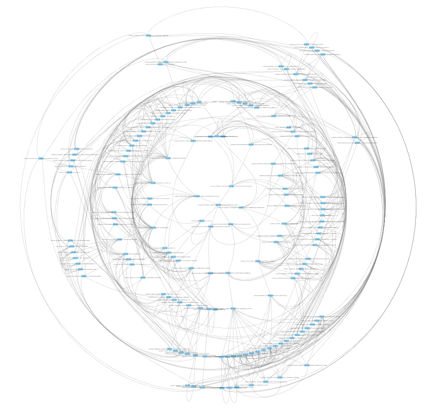Figure 1: Aggregated kNN graph obtained by aggregating three kNN graphs consutucted using three distance functions, abs_correlation, abs_spearmann, and abs_kendall.

An interesting property of the aggregated graph in Fig. 1 is that each edge is supported by at least 2 distance functions. Alternatively, one can aggregate the three graphs such that each edge is supported by one fixed base distance function (e.g., abs_correlation) plus at least one of the remaining two functions. Therefore, each edge in the resulting aggregated graph (Fig. 2) is supported by at least two functions such that one of them is abs_correlation.

Method 2 for constructing an undirected aggregated kNN graph

# Specify input/output files and parameters

# Output file
healthy_graph_file2 = './graphs/L6_healthy_aknng2.graphml'   # Output file for aggregated pkNN graphs

# Graph aggregation parameters
base_distance = abs_correlation
dists = [abs_spearmann, abs_kendall]   # distance functions
min_votes = 1

graphs = []
# Construct kNN-graphs using different distance fucntions
for dist in dists:
    nodes, a = get_knn_graph(df, k=num_neighbors, metric=dist)
    graphs.append(a.todense())

nodes, a = get_knn_graph(df, k=num_neighbors, metric=base_distance)
aggregated_graph,_ = filter_edges_by_votes(a.todense(), graphs, min)

# Save the constructed graph in an edge list format
save_graph(aggregated_graph, nodes, healthy_graph_file2)

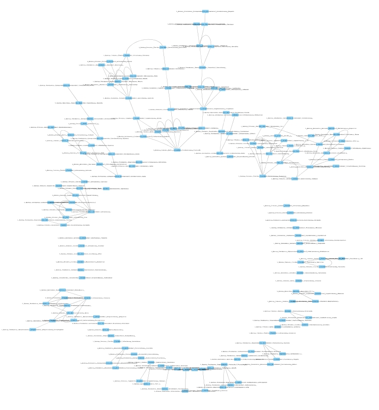Figure 2: Sparse base kNN graph (using abs_correlation) and remaining two graphs are used for filtering out unsupported edges.

It worths to mention that these two methods of aggregating graphs could also be applied to aggregate the following graphs:

<li> kNN graphs constructed with different <i>k</i> values</li>
<li> radius graphs rNN graphs with different <i>radius</i> values</i>
<li> different perturbed kNN graphs obtained using different T, c, k, or distance parameters</li>